Last summer (2015), as I put myself through the paces in this brilliant course by one of my personal heroes, Andrew Ng, I grew exceedingly confident about my ability to implement complex machine learning approaches (I blame credit Dr. Ng). Consequently, upon finishing the course, I jumped straight into [what I later realized was] the deep end by signing up for the Metis¹ Naive Bees Classifier challenge, hosted by DrivenData.org² .

Nevertheless, despite the fact that my main intention was just to get my hands dirty with machine learning code,  I quickly realized that my approach to training an algorithm to differentiate between the Bees genus was rather, well… naive: I was trying to extract the dominant colors from the training images, using either Principal Components Analysis or K-Means clustering; once done, I wanted to run a classifier on this much smaller subspace of features. This turned out to be an ill-informed strategy – too embarrassed to post the training error –  simply because… well, take a look at some of the training images for yourself:

Becoming harder to tell the Apis apart from Background (colors are pretty varied in background)

Way too many color variations in background!

Can you spot the Bombus bee? Took me a while!

A rare close up of the Apis (honey bee) sub species

[Click “Read More” to read how I explored Kmeans clustering on these images.]

Look at the enormous variations in color throughout the images. My strategy was doomed from the start because the algorithm wasn’t learning anything about the bees themselves, it was learning about the spread of colors in the entire image! Given that no two backgrounds in the training images look alike, well, you can guess at the dismal accuracy it might produce.

Looking back, however, it wasn’t all foolhardy, considering I at least managed to intricately acquaint myself with the K means algorithm as laid bare in Dr. Ng’s course, albeit in R. I wanted to write it out “manually” (without using the precompiled routine) just to solidify my intuition of how k-means works. As shown towards the end, using the precompiled k-means algorithm from the base stats package in R is way faster! Keep that in mind as you go through the steps below.

Objectives

• Extract common colors from an image using K-means algorithm
  • Code for each step of the basic K-means intuition;
  • Use the precompiled kmeans routine in base R’s stats package.

Image Data

The idea is that I’m able to extract the most common colors, or alternatively, compress the image to its main colors, on any image possible. I get to specify how many such color “clusters” I’m interested in compressing the image down to. I imagine that typically depends on the problem domain that you are trying to solve for. In this case, let’s say I’m interested in extracting the 5 most dominant colors from my input image.

Image Specs

To keep things manageable for now, I’m using a 200px by 200px image from the same Naive Bees Classifier competition’s training dataset. To the right, is what an input image looks like. My non-colorblind human eye can detect at least two or three shades of green, at least two shades of yellow, black, and white, and this is given my very weak training in the art of detecting colors. The K-means algorithm can be a lot more specific 🙂

The image itself is a 24-bit RGB image, which means that, for each pixel, of which there are 200*200 = 40,000, there are 3 unsigned integers giving us the intensity values of “red”, “green”, and “blue” colors. It takes 8 bits to represent each value between an intensity range of 0 and (2^8 – 1 ) 255, I get a total image physical size of (200 pixels * 200 pixels * 3 bytes/pixel) approximately 120,000 bytes, or around 120KB. The lossy JPEG compression, however, results in an actual storage size of an approximate average of 10KB per image, giving us a compression ratio of approximately 12x. Note how the size of the image starts to become a serious liability when we start dealing with images captured by modern smartphones (upwards of 16 Mega Pixels!) For now, I’ll deal with this nice 0.04 MP image size. I’ll be hoping to tackle larger images in the future. These specs aren’t really required for the exercise below, but it starts to become crucial, I imagine, when training on thousands of high quality images.

Read Image

The first step is reading in the image. I cheat a bit here and use a handy R library called “raster”:

library(raster)
 # read in some image; it's a (m*n)X(RGB) 2D matrix; each pixel is unrolled
# into its corresponding RGB value, rowise
  raw.imgs <- matrix(0, nrow=1, ncol=200*200*3)
#system.time(
raw.imgs <- t(sapply(tnames$id, function(X){
temp <- getValues(brick(paste0("/Users/ash/Downloads/Bees Data/images/train","/",paste0(X,".jpg"))))
c(temp[,1], temp[,2], temp[,3])
}))

I use the raster library to read in the image using the brick() function which reads the image in as a raster brick (layered raster values). getValues() returns the values of the raster brick in a nice matrix format that reflects the (in this case) RGB pixel values (0-255) in 3 columns, with a row dedicated to each pixel. To elaborate, if we have n pixels on each horizontal row of the image, that has m such rows, this gives us a total of m*n pixels. getValues() simply “rolls” the pixel values for the first row vertically (three intensities per pixel on each row of the matrix), then the second row of pixels, and so on for m rows. This gives us a total of m*n rows, each representing a pixel of the image going from left to right, top down.

I then proceed to normalize my image matrix by dividing by 255 just so I have values between 0 and 1. Although this isn’t required in the manual calculations it’s probably a good idea to normalize if the intent is to pass it to some algorithm down the line.

Finding Color Clusters

Now that I have the image matrix, I can begin figuring out the common color clusters in the image. How many clusters I’m looking for is entirely up to me and the problem domain in which I’m processing this image. To start with, let’s just say that I want my algorithm to “recognize” only the top five colors in my image.

K Means Steps

Thanks to Andrew Ng’s awesome course (have I mentioned this?) and phenomenal teaching style, I knew exactly how to go about this in Matlab. But I love R! So I re-did this in R without the use of packages just to solidify my intuition.

Step 1: Initialize Random Cluster Centroids

 # 1. Initiate k random cluster centroids
## pick k random indices from img and assign to centroid

 k <- 5
centroids <- as.matrix(img[sample(1:img.dim[1], size=k, replace=F), ]) 
  # initialize centroid index vectors
c.idx <- matrix(0, ncol=2, nrow=img.dim[1])
c.idx[,2] <- 99 #temp value to enter loop below

Using the sample() function, I’ve randomly extracted k indices from the image matrix. These  values will serve as my starting “centers” for my yet-to-be-found color clusters.

centroids above should result in an kx3 matrix of RGB color intensities, representing k random guesses at the color clusters that I’m interested in obtaining.

Steps 2 and 3: Cluster Assignment and Move Centroids

Now that I have k randomly initiated centers of our not-yet-found clusters, I begin the process of finding said clusters as follows:

1. For all pixels, compute the Euclidean distance between each pixel and each centroid. I’ll make do with the sum of squares which will capture the same idea.
2. Find the index position of the closest centroid to each pixel. I want to minimize the distance function between each pixel and each k centroid.
3. Once I have this map for every pixel, “move” each centroid to the mean distance of all the image pixels that are mapped to it.
4.  Repeat 1-3 above until the centroids can’t “move” anymore, i.e. every pixel is now mapped to its closest centroid.

  #loop until all pixel centroid assignments are identical on subsequent iteration
#WARNING: could loop for a while since I haven't set a cap on iterations!
 while (!identical(c.idx[,1], c.idx[,2])){
c.idx[,1] <- c.idx[,2]
# 2. CLUSTER ASSIGNMENT STEP:
## Compute sum of squares distance from each pixel row to each
## centroid: min k ||imagepixel - centroid_k||^2
## Track Closest Centroid: Index vector c.idx has indices of closest centroid
## to each image pixel

#slow...
  c.idx[,2] <- apply(img, 1, function(Z){

which.min(apply(centroids[(nrow(centroids)-(k-1)):nrow(centroids),], 1, function(X){
sum((Z - X)^2)
}))
})

# 3. MOVE CENTROID STEP:
## move each centroid to the average distance of all pixels to which this
## centroid is mapped (in the centroid index vector)
## c.idx correponds to each row of img; contains index of centroid
## you want centroid = mean of all cells of img that correspond to c.idx == k

centroids <- rbind(centroids, t(sapply(unique(c.idx[,2]), function(X){
colMeans(img[which(c.idx[,2]==X),])
})))

}

Step 2 above takes a little over 1.5 seconds on every iteration because each time it has to go through all m*n pixel rows, compute the distance from k centroid, extract the index of the closest centroid, and assign it to a column of the index matrix I created. This whole loop took about 1.5 minutes! Perhaps a parallelized implementation of step 2 is in order, along with a gloss over from the R experts on the appropriate use of the apply functions (I suspect it might be making copies of the matrix during the assignment and that there’s a more efficient way to achieve the same).

Results

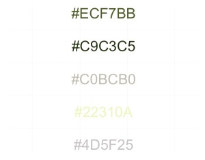
That’s it! The centroids matrix contains the RGB decomposition of k color clusters. This is an example of the color clusters it found for the input image above, coded to their hex code and colors:

The R code that makes this plot happen:

library(ggplot2)

#get k last rows in centroid matrix
#plot hex colors 
 colordf <- data.frame(x=rep(1,k), y=k:1,
colors=apply(centroids[(nrow(centroids)-(k-1)):nrow(centroids),],1,function(X){
rgb(red=X[1], green=X[2], blue=X[3])
}))
 #plot hex codes
ggplot(colordf, 
 aes(x,y,label=colors)) +
 geom_text(aes(col=colors),size=15) +
 scale_color_manual(values=as.character(colordf$colors)) +
 theme(legend.position='none', 
 axis.title=element_blank(),
 axis.ticks=element_blank(),
 axis.text=element_blank(),
 panel.border=element_blank(),
 panel.background=element_blank())

And, if you’re curious, these are the random guesses that the algorithm started out with:

Displaying Compressed Image

The fun wouldn’t be complete if I didn’t actually show what the image looks like when each pixel is replaced with the closest color centroid that the algorithm found: The “compressed” color image…

And this is how I went about assigning the closest centroids for each pixel to that pixel location, to generate the image above:

# Now that we have the top k colors to represent the image, we want
# to assign to each image cell its closest centroid value, thus compressing
# our image to a k color image.

# assign closest centroids color values for each pixel to new image

 img.comp <- t(sapply(c.idx[,2], function(X){
centroids[nrow(centroids)-(k-X),]
}))

img.df &lt;- data.frame(
 x = rep(1:200, times=200),
 y = rep(200:1, each=200),
 r = as.vector(img.comp[,1]),
 g = as.vector(img.comp[,2]),
 b = as.vector(img.comp[,3])
 )
#display
g <- ggplot(img.df, aes(x=x,y=y))
g + geom_point(color=rgb(img.df[c('r','g','b')]))

PreCompiled K Means in R

Now let’s actually look into R’s vast statistical arsenal and use a nicely packaged and optimized K-means routine, courtesy of the already included stats library. It literally takes a few lines of code to do this, assuming all the image processing is done! I’m using only 1 random start, although Dr. Ng recommends conducting multiple random starts of the algorithm to allow it a greater chance to find the global maxima for each cluster.

system.time(
kmclusts <- kmeans(img, k, iter.max = 500, nstart = 1, trace=FALSE)
)

So that totally embarrassed my manual steps by running in a fifth of a second (0.05 second)!!!

And did it converge correctly? You bet it did!

print(rgb(kmclusts$centers))

Produces: “#4D5122” “#7E7646” “#A9AB7A” “#252F10” “#DBD9CD”

Exactly the same clusters as the results above!

For the Future

Now that I know exactly how the basic principle works, I’ll gladly be using the precompiled kmeans routine in R. But my ego’s left a bit bruised with the precompiled package showing at least a 1600x improvement in performance. So I’ll concede defeat, but ruminate over the following for the future:

• Difference in the “Hartigan-Wong” algorithm used by the package versus this basic approach;
• How I can optimize the basic approach with better R code;
• How I can parallelize the basic approach

Basically, I’ll be wondering how to best optimize the basic approach to improve on the benchmark set by the stats::kmeans() routine. Perhaps a part II of this post beckons.

 End of Post.

Footnotes:
¹ also the folks who're training me to be a more hardcore Data Scientist right now (summer 2016), although I prefer to think of myself as more of a Machine Learning Engineer, if anything. 
² DrivenData.org are the "Kaggle" for social good, for me.